Numpy (Numerical Python) and Matplotlib

From http://www.numpy.org/:

NumPy is the fundamental package for doing scientific computing with Python. It contains among other things:

• a powerful N-dimensional array object
• sophisticated (broadcasting) functions
• tools for integrating C/C++ and Fortran code
• useful linear algebra, Fourier transform, and random number capabilities

Besides its obvious scientific uses, Numpy can also be used as an efficient multi-dimensional container of generic data. Arbitrary data-types can be defined. This allows NumPy to seamlessly and speedily integrate with a wide variety of databases.

Numpy is the standard go-to for manipulating numerical data in python. It lets you create matrices, do matrix operations, pretty printing, and so much more.

Once we’ve carried out some calculations on our data with Numpy, it’s likely that we’ll want to visualize this somehow. A widely used library for doing this is matplotlib:

From http://matplotlib.org/index.html:

matplotlib is a python 2D plotting library which produces publication quality figures in a variety of hardcopy formats and interactive environments across platforms. matplotlib can be used in python scripts, the python and ipython shell (ala MATLAB®* or Mathematica®†), web application servers, and six graphical user interface toolkits.

Lets get started by importing numpy and matplotlib.pyplot.

# and import necessary libraries
import numpy as np
import matplotlib.pyplot as plt

# Allows plots to display in the notebook
%matplotlib inline

Let’s begin by using numpy to do some mathematics for us! First let’s create a list of numbers between $[-2\pi, 2\pi]$, then calculate the sine of these numbers.

# Make a list of 100 numbers between -2*pi and 2*pi
x_values = np.linspace(-2 * np.pi, 2 * np.pi, 100)

print(x_values)

[-6.28318531 -6.15625227 -6.02931923 -5.9023862  -5.77545316 -5.64852012
 -5.52158709 -5.39465405 -5.26772102 -5.14078798 -5.01385494 -4.88692191
 -4.75998887 -4.63305583 -4.5061228  -4.37918976 -4.25225672 -4.12532369
 -3.99839065 -3.87145761 -3.74452458 -3.61759154 -3.4906585  -3.36372547
 -3.23679243 -3.10985939 -2.98292636 -2.85599332 -2.72906028 -2.60212725
 -2.47519421 -2.34826118 -2.22132814 -2.0943951  -1.96746207 -1.84052903
 -1.71359599 -1.58666296 -1.45972992 -1.33279688 -1.20586385 -1.07893081
 -0.95199777 -0.82506474 -0.6981317  -0.57119866 -0.44426563 -0.31733259
 -0.19039955 -0.06346652  0.06346652  0.19039955  0.31733259  0.44426563
  0.57119866  0.6981317   0.82506474  0.95199777  1.07893081  1.20586385
  1.33279688  1.45972992  1.58666296  1.71359599  1.84052903  1.96746207
  2.0943951   2.22132814  2.34826118  2.47519421  2.60212725  2.72906028
  2.85599332  2.98292636  3.10985939  3.23679243  3.36372547  3.4906585
  3.61759154  3.74452458  3.87145761  3.99839065  4.12532369  4.25225672
  4.37918976  4.5061228   4.63305583  4.75998887  4.88692191  5.01385494
  5.14078798  5.26772102  5.39465405  5.52158709  5.64852012  5.77545316
  5.9023862   6.02931923  6.15625227  6.28318531]

We’ve done a few things here: we used numpy’s own linspace function to create the list of 100 numbers, starting from $-2\pi$ and ending with $2\pi$. We did this using numpy’s own value of $\pi$, np.pi.

Now lets make a number list of numbers, equal to $y = \sin(x)$.

y_values = np.sin(x_values)
print(y_values)

[ 2.44929360e-16  1.26592454e-01  2.51147987e-01  3.71662456e-01
  4.86196736e-01  5.92907929e-01  6.90079011e-01  7.76146464e-01
  8.49725430e-01  9.09631995e-01  9.54902241e-01  9.84807753e-01
  9.98867339e-01  9.96854776e-01  9.78802446e-01  9.45000819e-01
  8.95993774e-01  8.32569855e-01  7.55749574e-01  6.66769001e-01
  5.67059864e-01  4.58226522e-01  3.42020143e-01  2.20310533e-01
  9.50560433e-02 -3.17279335e-02 -1.58001396e-01 -2.81732557e-01
 -4.00930535e-01 -5.13677392e-01 -6.18158986e-01 -7.12694171e-01
 -7.95761841e-01 -8.66025404e-01 -9.22354294e-01 -9.63842159e-01
 -9.89821442e-01 -9.99874128e-01 -9.93838464e-01 -9.71811568e-01
 -9.34147860e-01 -8.81453363e-01 -8.14575952e-01 -7.34591709e-01
 -6.42787610e-01 -5.40640817e-01 -4.29794912e-01 -3.12033446e-01
 -1.89251244e-01 -6.34239197e-02  6.34239197e-02  1.89251244e-01
  3.12033446e-01  4.29794912e-01  5.40640817e-01  6.42787610e-01
  7.34591709e-01  8.14575952e-01  8.81453363e-01  9.34147860e-01
  9.71811568e-01  9.93838464e-01  9.99874128e-01  9.89821442e-01
  9.63842159e-01  9.22354294e-01  8.66025404e-01  7.95761841e-01
  7.12694171e-01  6.18158986e-01  5.13677392e-01  4.00930535e-01
  2.81732557e-01  1.58001396e-01  3.17279335e-02 -9.50560433e-02
 -2.20310533e-01 -3.42020143e-01 -4.58226522e-01 -5.67059864e-01
 -6.66769001e-01 -7.55749574e-01 -8.32569855e-01 -8.95993774e-01
 -9.45000819e-01 -9.78802446e-01 -9.96854776e-01 -9.98867339e-01
 -9.84807753e-01 -9.54902241e-01 -9.09631995e-01 -8.49725430e-01
 -7.76146464e-01 -6.90079011e-01 -5.92907929e-01 -4.86196736e-01
 -3.71662456e-01 -2.51147987e-01 -1.26592454e-01 -2.44929360e-16]

Here, we passed in our list of x_values to numpy’s built in np.sin function. Numpy then calculated the sine of each number in this list, and returned us another list which we stored in the variable y_values.

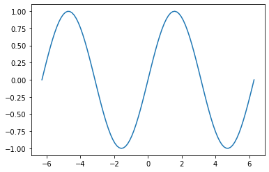
Great! Let’s create a plot of these values so we can see what they look like.

plt.plot(x_values, y_values)
plt.show()

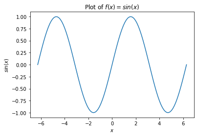
So that worked, but let’s make our plot a little more informative

plt.title("Plot of $f(x) = sin(x)$")     # put a title on the plot
plt.xlabel("$x$")                        # label the x axis
plt.ylabel("$sin(x)$")                   # label the y axis
plt.plot(x_values, y_values)
plt.show()

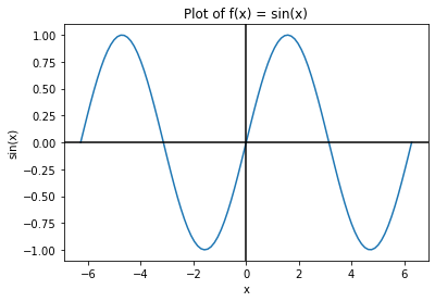
That looks pretty good. What about adding in the axes?

plt.title("Plot of f(x) = sin(x)")
plt.xlabel("x")
plt.ylabel("sin(x)")
plt.plot(x_values, y_values)
plt.axhline(y=0, color='k')
plt.axvline(x=0, color='k')
plt.show()

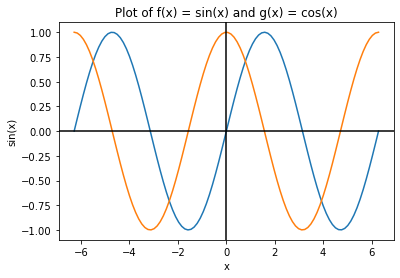
What about plotting more than one function at a time? Easy!

plt.title("Plot of f(x) = sin(x) and g(x) = cos(x)")
plt.xlabel("x")
plt.ylabel("sin(x)")
plt.plot(x_values, y_values)
plt.plot(x_values, np.cos(x_values))
plt.axhline(y=0, color='k')
plt.axvline(x=0, color='k')
plt.show()

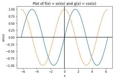
We can also turn the lines from solid to dashed quite easily.

plt.title("Plot of f(x) = sin(x) and g(x) = cos(x)")
plt.xlabel("x")
plt.ylabel("sin(x)")
plt.plot(x_values, y_values)
plt.plot(x_values, np.cos(x_values), '--') # The '--' changes the line style to dashed
plt.axhline(y=0, color='k')               # The color 'k' is black, if you wondered.
plt.axvline(x=0, color='k')
plt.show()

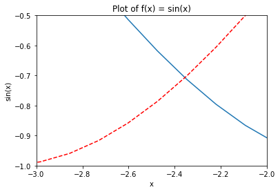
What if we wanted to zoom in on only a certain section of our plot? We can do that by changing the axis limits.

plt.title("Plot of f(x) = sin(x)")
plt.xlabel("x")
plt.ylabel("sin(x)")
plt.plot(x_values, y_values)
plt.plot(x_values,np.cos(x_values), '--r') 
plt.axhline(y=0, color='k') 
plt.axvline(x=0, color='k')
plt.xlim([-3,-2])            # change the limits of the x axis
plt.ylim([-1.0,-0.5])        # change the limits of the y axis
plt.show()

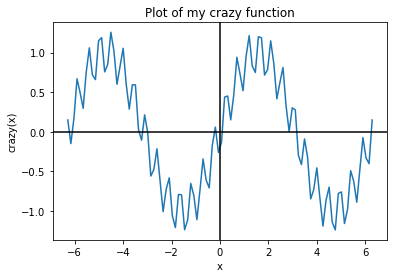
Just for fun, lets try and create a crazy function and just see what it looks like.

plt.title("Plot of my crazy function")
plt.xlabel("x")
plt.ylabel("crazy(x)")
plt.plot(x_values, 0.3 * np.cos(20.0 * np.pi * x_values) + np.sin(x_values))
plt.axhline(y=0, color='k')
plt.axvline(x=0, color='k')
plt.show()

What if I’m really proud of my work and want to save it forever so that I never lose it? Maybe print it out and put it on the fridge. We can do that too.

plt.title("Plot of my crazy function")
plt.xlabel("x")
plt.ylabel("crazy(x)")
plt.plot(x_values, 0.3 * np.cos(20.0 * np.pi * x_values) + np.sin(x_values))
plt.axhline(y=0, color='k')
plt.axvline(x=0, color='k')
plt.savefig('crazy.png')    # This line saves the figure to the hard disk
plt.show()

Let’s look at more of what numpy can do!

Numpy can be used to create arrays. These are like Python’s in-built lists, but much more powerful. To see this, let’s try adding two lists then repeat this with two arrays.

a_list = [4, 6, 8]
b_list = [1, 8, 1]

a_list + b_list

[4, 6, 8, 1, 8, 1]

a_array = np.array([4, 6, 8])
b_array = np.array([1, 8, 1])

a_array + b_array

array([ 5, 14,  9])

What happened here? When we added the two lists, Python simply concatenated the second list onto the end of the first one. However, when we added the two arrays, numpy added the two arrays together element-by-element. This is often extremely useful when manipulating data, and saves us from having to write loops to iterate over the elements individually. As a bonus, it also tends to be much more computationally efficient to do calculations this way in Python instead of looping over the arrays by hand (thanks to some clever numpy stuff).

Numpy also makes it much easier to create and manipulate multi-dimensional arrays:

A = np.array([[1, 2, 1],
              [4, 5, 6],
              [7, 8, 9]])  # note: the extra lines I've added here are not necessary, but do make my code at lot more readable!

print(A)

[[1 2 1]
 [4 5 6]
 [7 8 9]]

A is a 2d array. We can find out its dimensions by printing out its shape, and find its total number of elements by printing its size:

print(A.shape)
print(A.size)

(3, 3)
9

Let’s create a new array by subtracting 5 from all the elements of A:

B = A - 5
print(B)

[[-4 -3 -4]
 [-1  0  1]
 [ 2  3  4]]

Just as with the 1d arrays, we can add, subtract, multiply, divide, etc these two arrays together, and numpy will carry out these calculations element-by-element:

A * B

array([[-4, -6, -4],
       [-4,  0,  6],
       [14, 24, 36]])

What about accessing elements of these 2d arrays? We can do this using a comma-separated list. The first index refers to the outermost dimension (here which of the lists in our list of arrays), then the second the inner dimension (here which element of that list).

print(A[0,1])  # 0th row, 1st column

print(B[:, 2]) # this will print the entire 2nd column

2
[-4  1  4]

A couple of particularly useful commands are zeros and ones. These will create arrays full of 0s and 1s of the shape provided

np.zeros((3,3))   # a 2d 3 x 3 array of 0s

array([[0., 0., 0.],
       [0., 0., 0.],
       [0., 0., 0.]])

np.ones((2,2,2))  # a 3d 2 x 2 x 2 array of 1s

array([[[1., 1.],
        [1., 1.]],

       [[1., 1.],
        [1., 1.]]])

Linear algebra with numpy

In your school math lessons, you may have come across matrices and linear algebra. Numpy arrays can be used for this as well!

Firstly, let’s create an identity matrix.

$$I = \begin{pmatrix} 1 & 0 & 0 \\ 0 & 1 & 0 \\ 0 & 0 & 1 \end{pmatrix}$$

my_eye = np.eye(3)

print(my_eye)

[[1. 0. 0.]
 [0. 1. 0.]
 [0. 0. 1.]]

Matrix matrix multiplication however, is not done with the asterisk (*).

A * my_eye

array([[1., 0., 0.],
       [0., 5., 0.],
       [0., 0., 9.]])

As we’ve seen before, this just does element-wise multiplication. Each value inside A was multiplied by the corresponding value inside my_eye, which was not what we wanted here!

To do true matrix-matrix multiplication, we need to use the @ symbol.

A @ my_eye

array([[1., 2., 1.],
       [4., 5., 6.],
       [7., 8., 9.]])

We can also do some other matrix operations in numpy. Many of these are contained within the linalg sub-library. For example, we can find the inverse of a matrix using np.linalg.inv:

np.linalg.inv(A)

array([[-0.5       , -1.66666667,  1.16666667],
       [ 1.        ,  0.33333333, -0.33333333],
       [-0.5       ,  1.        , -0.5       ]])

Let’s create a vector (essentially a 1d matrix).

b = np.array([1,3,5])

We can then use another of these linear algebra functions to solve this system of equations (in matrix form):

$$A x = b$$

np.linalg.solve(A,b)

array([3.33333333e-01, 3.33333333e-01, 7.53365624e-17])

By luck, our linear system has a unique solution.

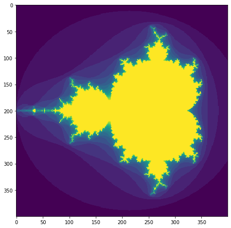
As a quick example to finish up, let’s use numpy and matplotlib to create a fractal image of the Mandelbrot set (if you’re unfamiliar with fractals, they are super cool - read more about them here). This code was pulled directly from numpy’s tutorial page.

import numpy as np
import matplotlib.pyplot as plt
def mandelbrot(h, w, maxit=20):
    """
    Returns an image of the Mandelbrot fractal of size (h,w).
    """
    y , x = np.ogrid[-1.4:1.4:h*1j, -2:0.8:w*1j]
    c = x + y * 1j
    z = c
    divtime = maxit + np.zeros(z.shape, dtype=int)

    for i in range(maxit):
        z = z**2 + c
        diverge = z * np.conj(z) > 2**2            
        div_now = diverge & (divtime==maxit)  
        divtime[div_now] = i                  
        z[diverge] = 2                        
    
    return divtime

plt.figure(figsize=(8,8))
plt.imshow(mandelbrot(400,400))
plt.show()

Practice

Array arithmetic

Let’s do some mathematics with numpy arrays. Below we’ve defined two arrays, A and B. Compute the following quantities:

1. add A to B element wise (so add the first element of A to the first element of B etc.)
2. subtract the elements of A from the elements of B
3. Multiply the arrays element-by-element
4. Square the elements of A
5. Calculate the exponential of the elements of A (so $\exp A_ij$ for all $i,j$)
6. Treating them as matrices, now multiply A by B
7. Again treating them as matrices, divide A by B
8. Calculate square of the matrix A

A = np.array([[1, 6, 1],
              [8, 6, 1],
              [0, 2, 7]])

B = np.array([[0, 1, 7],
              [12,9, 2],
              [1, 0, 1]])

A + B

array([[ 1,  7,  8],
       [20, 15,  3],
       [ 1,  2,  8]])

A - B

array([[ 1,  5, -6],
       [-4, -3, -1],
       [-1,  2,  6]])

A * B

array([[ 0,  6,  7],
       [96, 54,  2],
       [ 0,  0,  7]])

A**2

array([[ 1, 36,  1],
       [64, 36,  1],
       [ 0,  4, 49]])

np.exp(A)

array([[2.71828183e+00, 4.03428793e+02, 2.71828183e+00],
       [2.98095799e+03, 4.03428793e+02, 2.71828183e+00],
       [1.00000000e+00, 7.38905610e+00, 1.09663316e+03]])

A @ B

array([[73, 55, 20],
       [73, 62, 69],
       [31, 18, 11]])

np.linalg.solve(A, B)

array([[ 1.71428571,  1.14285714, -0.71428571],
       [-0.325     , -0.025     ,  1.325     ],
       [ 0.23571429,  0.00714286, -0.23571429]])

np.linalg.matrix_power(A, 2)

array([[49, 44, 14],
       [56, 86, 21],
       [16, 26, 51]])

Plotting

In your math classes at school, you have probably come across simultaneous equations. Here we have 2 or more variables (e.g. $x$ and $y$) which are described by 2 or more equations. By solving the equations simultaneously, we can find the values of the variables.

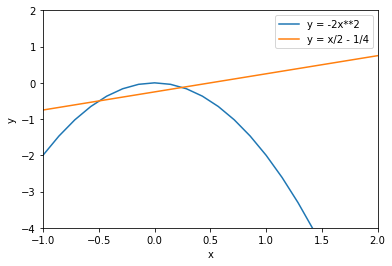
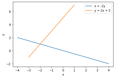
One way of solving simultaneous equations is by plotting the functions and finding the point way they intersect. Try that here for the following pairs of equations.

1. Try plotting between $-3 \leq x \leq 1$ and $-2 \leq y \leq 2$: $x + 2 y = 0$

$$2 x - y + 5 = 0$$

1. Try plotting between $-2 \leq x \leq 5$ and $-2 \leq y \leq 5$ $x^2 + 0.5 y = 0$ $4y - 2x + 1 = 0$

y = np.linspace(-2, 2)
x = - 2 * y

x2 = np.linspace(-3, 1)
y2 = 2 * x2 + 5

plt.plot(x, y, label='x = -2y')
plt.plot(x2, y2, label='y = 2x + 5')
plt.xlabel('x')
plt.ylabel('y')
plt.legend()

<matplotlib.legend.Legend at 0x1136d3f28>

x = np.linspace(-2, 5)
y = -2 * x**2

x2 = np.linspace(-2, 5)
y2 = 1/2 * x - 1/4

plt.plot(x, y, label='y = -2x**2')
plt.plot(x2, y2, label='y = x/2 - 1/4')
plt.xlabel('x')
plt.ylabel('y')
plt.xlim([-1, 2])
plt.ylim([-4, 2])
plt.legend()

<matplotlib.legend.Legend at 0x1133f6c18>

Back to day 3