Day 3 Review

Yesterday we looked at strings, numpy, matplotlib and turtles.

(Note: if you’re wondering why we looked at turtles, this was mainly to illustrate how libraries work. Many people write their own Python code and package it up as libraries, available for people to download using PyPI (the Python Package Index) and/or conda. So now you’ve seen how to use the turtles library, you should be able to download other libaries and use them in your own code!)

Strings

# Define a string
my_string = "Hi! I'm a string!"
print(my_string)

Hi! I'm a string!

# Access an element
an_element = my_string[4]
print(an_element)

I

# Slice it up 
a_slice = my_string[:3]
print(a_slice)

Hi!

# Reverse it
reversed_string = my_string[::-1]
print(reversed_string)

!gnirts a m'I !iH

# add strings 
added_string = my_string + " Who are you?"
print(added_string)

Hi! I'm a string! Who are you?

# find the length
len(my_string)

17

# make it lower case
my_string.lower()

"hi! i'm a string!"

# make it upper case
my_string.upper()

"HI! I'M A STRING!"

# split it into a list of strings
my_string.split()

['Hi!', "I'm", 'a', 'string!']

# replace some characters 
my_string.replace("i", "z")

"Hz! I'm a strzng!"

Numpy & matplotlib

# import the libraries 
import numpy as np
import matplotlib.pyplot as plt

# create a numpy array
my_array = np.array([1,2,3])
my_array

array([1, 2, 3])

# adding numpy arrays adds them element-wise (whereas adding lists joins them together)
my_second_array = np.array([4,5,6])

my_array + my_second_array

array([5, 7, 9])

# we can also subtract, multiply and divide element-wise
print(my_array - my_second_array)
print(my_array * my_second_array)
print(my_array / my_second_array)

[-3 -3 -3]
[ 4 10 18]
[0.25 0.4  0.5 ]

# if we multiply by a number, it will multiply element-wise rather than copying the list n-times
my_array * 124.234

array([124.234, 248.468, 372.702])

# we can do all of the above for multi-dimensional arrays 
my_2d_array = np.array([[1,2,3],
                        [4,5,6],
                        [7,8,9]])
my_2d_array

array([[1, 2, 3],
       [4, 5, 6],
       [7, 8, 9]])

my_2d_array * 5

array([[ 5, 10, 15],
       [20, 25, 30],
       [35, 40, 45]])

# we can access elements of an nd array using a comma-separated list
my_2d_array[1,0]

4

# we can find the shape of the array and the number of elements in it using the shape and size functions
print(my_2d_array.size)
print(my_2d_array.shape)

9
(3, 3)

# numpy has lots of built-in mathematical operations like the trigonometric functions
# it also knows pi, so let's calculate sine between 0 and 2*pi
# we first define a 1d array with 50 equally spaced values between 0 and 2*pi using linspace
x = np.linspace(0, 2 * np.pi)
x

array([0.        , 0.12822827, 0.25645654, 0.38468481, 0.51291309,
       0.64114136, 0.76936963, 0.8975979 , 1.02582617, 1.15405444,
       1.28228272, 1.41051099, 1.53873926, 1.66696753, 1.7951958 ,
       1.92342407, 2.05165235, 2.17988062, 2.30810889, 2.43633716,
       2.56456543, 2.6927937 , 2.82102197, 2.94925025, 3.07747852,
       3.20570679, 3.33393506, 3.46216333, 3.5903916 , 3.71861988,
       3.84684815, 3.97507642, 4.10330469, 4.23153296, 4.35976123,
       4.48798951, 4.61621778, 4.74444605, 4.87267432, 5.00090259,
       5.12913086, 5.25735913, 5.38558741, 5.51381568, 5.64204395,
       5.77027222, 5.89850049, 6.02672876, 6.15495704, 6.28318531])

# now calculate sine
y = np.sin(x)
y

array([ 0.00000000e+00,  1.27877162e-01,  2.53654584e-01,  3.75267005e-01,
        4.90717552e-01,  5.98110530e-01,  6.95682551e-01,  7.81831482e-01,
        8.55142763e-01,  9.14412623e-01,  9.58667853e-01,  9.87181783e-01,
        9.99486216e-01,  9.95379113e-01,  9.74927912e-01,  9.38468422e-01,
        8.86599306e-01,  8.20172255e-01,  7.40277997e-01,  6.48228395e-01,
        5.45534901e-01,  4.33883739e-01,  3.15108218e-01,  1.91158629e-01,
        6.40702200e-02, -6.40702200e-02, -1.91158629e-01, -3.15108218e-01,
       -4.33883739e-01, -5.45534901e-01, -6.48228395e-01, -7.40277997e-01,
       -8.20172255e-01, -8.86599306e-01, -9.38468422e-01, -9.74927912e-01,
       -9.95379113e-01, -9.99486216e-01, -9.87181783e-01, -9.58667853e-01,
       -9.14412623e-01, -8.55142763e-01, -7.81831482e-01, -6.95682551e-01,
       -5.98110530e-01, -4.90717552e-01, -3.75267005e-01, -2.53654584e-01,
       -1.27877162e-01, -2.44929360e-16])

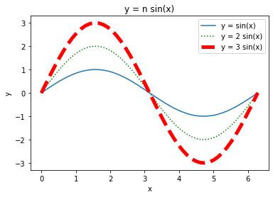
# matplotlib has lots of plotting functions for visualizing data
# here we'll do a line plot

plt.plot(x, y, label='y = sin(x)') # the label argument will be used in the legend

# we can change the line color and style in this compact way (to a green dotted line)
plt.plot(x, 2 * y, 'g:', label='y = 2 sin(x)') 

# this is another way of setting the line color, style and width
plt.plot(x, 3 * y, c='red', ls='--', lw='5', label='y = 3 sin(x)') 

plt.xlabel('x') # always label your axes!
plt.ylabel('y')
plt.title('y = n sin(x)')

plt.legend() # remember to call this or else it won't print the legend

<matplotlib.legend.Legend at 0x1171298d0>

Turtles

# import a module 
import turtle

# access a module function 
# here we shall create a window 
window = turtle.Screen()

# make a turtle and get it to draw a circle
ned = turtle.Turtle()
ned.circle(4)

# say goodbye to ned
window.bye()

Back to day 4